5. Linear and Logistic regression with JAX#
In this lecture, we will try to build a simple model of linear and logistic regression using JAX and it’s auto-grad capabilities.
5.1. Linear regression#
Linear regression is a statistical method used to model the relationship between a dependent variable and one or more independent variables. It assumes a linear relationship, aiming to find the best-fit line that minimizes the difference between predicted and actual values.
With a single independent variable, it’s expressed as \( y = Wx + b \), where \(y\) is the dependent variable, \(x\) is the independent variable, \(W\) is the slope, and \(b\) is the intercept. Linear regression is widely applied in various fields for prediction, analysis, and understanding relationships between variables.
Let’s start with the imports
import jax
import jax.numpy as jnp
import matplotlib.pyplot as plt
5.1.1. Data preparation#
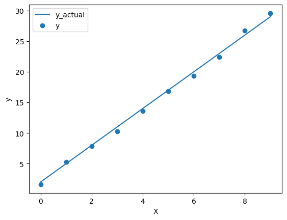
We will create a some random data set that will use for training our model.
Here, we have assume that \(W=3\) and \(b=2\).
We will take 10 data points as \(X\) and compute y_actual using \(Wx+b\) and then add some random noise using normal distribution to compute our \(y\).
actual_W = 3.0
actual_b = 2.0
num_points = 10

key = jax.random.PRNGKey(0)
X = jnp.arange(num_points).reshape((num_points, 1))
y_actual = actual_W * X + actual_b
noise = jax.random.normal(key, (num_points, 1))
y = y_actual + noise
plt.plot(X, y_actual, label='y_actual')
plt.scatter(X, y, label='y')
plt.xlabel('X')
plt.ylabel('y')
plt.legend()
plt.show()
Now, let’s define the following two functions
Forward Pass Function (
forward):The
forwardfunction takes inputxand model parametersparams(which include weightsWand biasesb) as input.It computes the forward pass of the neural network by performing a dot product between the input
xand the weightsW, and then adding the biasesb.The result is the output of the neural network.
Loss Function (
loss_fn):The
loss_fnfunction takes inputx, ground truth labelsy, and model parametersparamsas input.It first computes predictions using the
forwardfunction.Then, it computes the mean squared error loss between the predictions and the ground truth labels.
This loss function quantifies the discrepancy between the predicted and actual values, providing a measure of how well the model is performing on the given data.
# Forward pass
@jax.jit
def forward(params, x):
    return jnp.dot(x, params['W']) + params['b']

# Define loss function of linear regression
@jax.jit
def loss_fn(params, x, y):
    preds = forward(params, x)
    return jnp.mean((preds - y) ** 2)
We define a gradient function grad_fn using JAX’s grad function, which computes the gradients of a given function (in this case, the loss function loss_fn) with respect to its input arguments.
# Define gradient function
grad_fn = jax.jit(jax.grad(loss_fn))
Next, we define a training loop where we iterate over a fixed number of epochs (num_epochs). In each epoch, we compute the gradients of the loss function with respect to the model parameters using grad_fn. These gradients indicate the direction and magnitude of change needed to minimize the loss.
After computing the gradients, we update the model parameters (params['W'] and params['b']) using gradient descent. This involves subtracting a fraction of the gradients from the current parameter values, scaled by a learning rate (lr). The learning rate controls the size of the step taken in the parameter space during optimization.
# Define model parameters (Initialize them)
params = {
    'W': jax.random.normal(key, (1, 1)),
    'b': jnp.zeros((1,))
}
lr = 0.01
num_epochs = 1000
for epoch in range(num_epochs):
    # Compute gradients
    grads = grad_fn(params, X, y_actual)
    # Update parameters
    params['W'] -= lr * grads['W']
    params['b'] -= lr * grads['b']
print("Trained Parameters:")
print("W:", params['W'])
print("b:", params['b'])
Trained Parameters:
W: [[3.0008037]]
b: [1.9949604]
This is almost the same that we had assumed earlier while creating our dataset.
5.2. Logistic regression#
Logistic regression is a statistical method used for binary classification tasks. Unlike linear regression, it models the probability that a given input belongs to a particular class using the logistic function, which maps input values to the range [0, 1].
It estimates the coefficients of the decision boundary that separates the classes, making it a linear classifier.
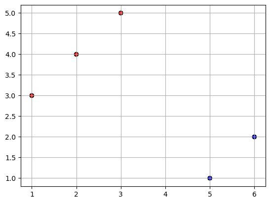
To begin with logistic regression, let’s create a small dataset with 5 data points.
key = jax.random.PRNGKey(10)

X = jnp.array([[1, 3], [3, 5], [2, 4], [6, 2], [5, 1]])
y = jnp.array([1, 1, 1, 0, 0]).reshape((5, 1))  # Binary labels (0 or 1)
# Plot dataset
plt.scatter(X[:, 0], X[:, 1], c=y, cmap='bwr', edgecolors='k')
plt.grid(True)
plt.show()
Now, let’s define the following functions
Sigmoid Activation Function:
The
sigmoidfunction is a mathematical function that maps any real-valued number to the range [0, 1].It is used as the activation function in logistic regression to squash the output of the linear combination of inputs to a probability value.
Forward Pass Function:
The
forwardfunction performs the forward pass of the logistic regression model.It takes the input features
xand the model parametersparams(including weightsWand biasb) as input.It computes the linear combination of input features and model weights, adds the bias term, and applies the sigmoid activation function to obtain the predicted probabilities.
Binary Cross-Entropy Loss Function:
The
loss_fnfunction calculates the binary cross-entropy loss between the predicted probabilities and the ground truth labelsy.It first computes the predicted probabilities using the
forwardfunction.It then calculates the cross-entropy loss, which measures the discrepancy between the predicted probabilities and the actual binary labels.
# Define the sigmoid activation function
@jax.jit
def sigmoid(x):
    return 1 / (1 + jnp.exp(-x))


# Forward pass function
@jax.jit
def forward(params, x):
    return sigmoid(jnp.dot(x, params['W']) + params['b'])


# Define binary cross-entropy loss function
@jax.jit
def loss_fn(params, x, y):
    preds = forward(params, x)
    return -jnp.mean(y * jnp.log(preds) + (1 - y) * jnp.log(1 - preds))
Next, similar to liner regression, we define a training loop where we iterate over a fixed number of epochs (num_epochs). In each epoch, we compute the gradients of the loss function with respect to the model parameters using grad_fn.
After computing the gradients, we update the model parameters (params['W'] and params['b']) using gradient descent. This involves subtracting a fraction of the gradients from the current parameter values, scaled by a learning rate (lr). The learning rate controls the size of the step taken in the parameter space during optimization.
# Define model parameters
params = {
    'W': jax.random.normal(key, (2, 1)),
    'b': jnp.zeros((1,))
}

# Define gradient function
grad_fn = jax.jit(jax.grad(loss_fn))
lr = 0.01
num_epochs = 1000
for epoch in range(num_epochs):
    # Compute gradients
    grads = grad_fn(params, X, y)
    # Update parameters using gradient descent
    params['W'] -= lr * grads['W']
    params['b'] -= lr * grads['b']

# Print trained parameters
print("Trained Parameters:")
print("W:", params['W'])
print("b:", params['b'])
Trained Parameters:
W: [[-1.0959495]
 [ 1.3521521]]
b: [0.42843798]
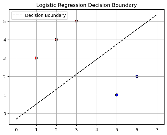
Let’s see how the predicted boundary looks like
plt.scatter(X[:, 0], X[:, 1], c=y, cmap='bwr', edgecolors='k')
W, b = params['W'], params['b']
# Generate x values for decision boundary line
x_values = jnp.linspace(X[:, 0].min() - 1, X[:, 0].max() + 1, 100)
# Compute y values for decision boundary line using the formula: W0*x + W1*y + b = 0
y_values = (-b - W[0] * x_values) / W[1]

# Plot decision boundary line
plt.plot(x_values, y_values, color='k', linestyle='--', label='Decision Boundary')
plt.title('Logistic Regression Decision Boundary')
plt.legend()
plt.grid(True)
plt.show()